
Timing Is Everything?
An Introduction to the Structured Life Course Modeling Approach
Joshua A. Goode
University of Michigan
November 13, 2026
Some Quick Notes
- Slides are available on my website.
- Please stop me with questions.
I’m Just a Padawan
Some materials have been adapted from Dr. Andrew Smith, who is a true Jedi Master. I am grateful and humbled by the opportunity to learn from him.
Outline
- Introduction to SLCMA
- Common SLCMA Hypotheses
- Manual Example
- The
slcmaPackage- Example 1: Complete Case Analysis with Binary Exposures
- Example 2: Imputed Data Analysis with Continuous Exposures and Covariates
- Important Issues to Keep in Mind
Part 6 · Time Permitting
Additional Topics
- Additional Hypotheses
- Extending SLCMA to New Analyses
- Choosing Recency Weights
Part 1 Introduction to SLCMA
Moving Beyond “Ever Exposed”
Where We Are
-
Narrow focus in much of the research
- Current exposure
- Ever exposed
-
We can do so much more
- Several large panel studies
- Many years of data
- A plethora of data types
- Really interesting questions/theory
-
Enter life course hypotheses
- Often tested, but rarely in a careful, structured way
What We Need
-
A careful, structured way to test life course hypotheses
- Compares competing hypotheses head to head
- Guards against false-positive results
- Scales to many exposures or outcomes
- Easy to use
- SLCMA can help!

What Is SLCMA?
Structured
Life
Course
Modeling
Approach

Which life course hypothesis best fits our data?
What Goes Into SLCMA?
SLCMA Steps
Fit a regression model for each single life course hypothesis of interest, as well as groups of compound hypotheses
Measure the goodness-of-fit of each model and select the best one
Calculate appropriate p-values for the selected model
Part 2 Common SLCMA Hypotheses
SLCMA Hypotheses
Big 3
- Sensitive Periods
- Accumulation
- Recency
Others
- Mobility
- Change
- Always Exposed
- Ever Exposed
Sensitive Periods \(\left(\mathit{SP} \text{ at } t_j\right)\)
- Idea: The developmental timing of an exposure has the strongest effect on the outcome at a specific time point due to heightened levels of plasticity or reprogramming
- Construct: Just the exposure variable at each age
- Exposure type: Binary or continuous
\[\mathit{SP}_j = x_j\]
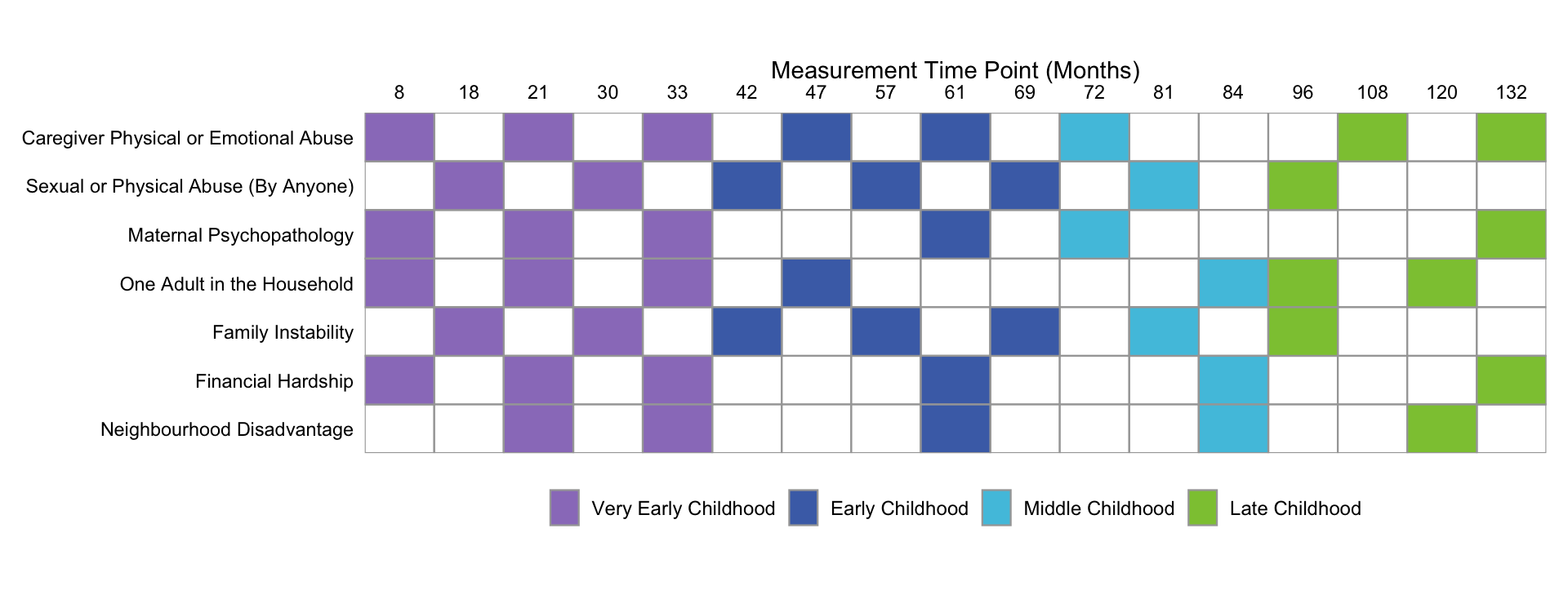
Sensitive Periods \(\left(\mathit{SP} \text{ at } t_j\right)\)
Multiple time points can also be grouped into more meaningful sensitive periods.
Accumulation \(\left(\mathit{Acc}\right)\)
- Idea: Every additional time point of exposure affects the outcome in a dose-response manner, independent of the exposure timing
- Construct: Add up the exposure variable across time points
- Exposure type: Binary or continuous
\[\mathit{Acc} = \sum_{j=1}^m{x_j}\]
Accumulation \(\left(\mathit{Acc}\right)\)
Example
| ID | Exp1 | Exp2 | Exp3 | Acc |
|---|---|---|---|---|
| 1 | 0 | 0 | 0 | \(0 + 0 + 0 = 0\) |
| 2 | 1 | 1 | 1 | \(1 + 1 + 1 = 3\) |
| 3 | 0 | 1 | 0 | \(0 + 1 + 0 = 1\) |
| 4 | 1 | 0 | 0 | \(1 + 0 + 0 = 1\) |
| 5 | 1 | 0 | 1 | \(1 + 0 + 1 = 2\) |
Recency \(\left(\mathit{Rec}\right)\)
- Idea: More proximal exposures (closer in time to the measurement of the outcome) are more strongly linked to the outcome than are more distal exposures
- Construct: Add up the products of each exposure variable multiplied by its age of observation
- Exposure type: Binary or continuous
\[\mathit{Rec} = \sum_{j=1}^m{\left(x_jt_j\right)}\]
Recency \(\left(\mathit{Rec}\right)\)
Example
| ID | Exp1 | Exp2 | Exp3 | Rec |
|---|---|---|---|---|
| 1 | 0 | 0 | 0 | \((0 \times 1) + (0 \times 2) + (0 \times 3) = 0\) |
| 2 | 1 | 1 | 1 | \((1 \times 1) + (1 \times 2) + (1 \times 3) = 6\) |
| 3 | 0 | 1 | 0 | \((0 \times 1) + (1 \times 2) + (0 \times 3) = 2\) |
| 4 | 1 | 0 | 0 | \((1 \times 1) + (0 \times 2) + (0 \times 3) = 1\) |
| 5 | 1 | 0 | 1 | \((1 \times 1) + (0 \times 2) + (1 \times 3) = 4\) |
Part 3 Manual Example
Manual Example Simulate Example Data
Manual Example Simulate Example Data
# set seed
set.seed(1234)

# simulate exposure & outcome data
n <- c(141, 20, 88, 80, 40, 35, 317, 367)
y <- c(28.7, 27.5, 29.1, 27.8, 28.3, 27.1, 27.6, 26.0)
se <- c(0.5, 1.1, 0.7, 0.7, 0.8, 0.9, 0.3, 0.2)
sp04 <- rep(c(0, 1, 0, 0, 1, 1, 0, 1), times = n)
sp26 <- rep(c(0, 0, 1, 0, 1, 0, 1, 1), times = n)
sp43 <- rep(c(0, 0, 0, 1, 0, 1, 1, 1), times = n)
e <- lm(rnorm(sum(n)) ~ sp04 * sp26 * sp43)$residuals
y <- rep(y, n) + rep(se * sqrt(n), n) * e / sd(e)

# create data frame
dats_bin <- data.frame(cbind(y, sp04, sp26, sp43))

# clean up
rm(n, y, se, sp04, sp26, sp43, e)Manual Example Step 1: Fit Models
Which single hypothesis best fits our data?
Call:
lm(formula = y ~ sp04, data = dats_bin)

Residuals:
     Min       1Q   Median       3Q      Max
-21.6360  -3.3888  -0.1199   3.0812  20.1639

Coefficients:
            Estimate Std. Error t value Pr(>|t|)
(Intercept)  28.0842     0.2092 134.219  < 2e-16 ***
sp04         -1.7368     0.3211  -5.409  7.8e-08 ***
---
Signif. codes:  0 '***' 0.001 '**' 0.01 '*' 0.05 '.' 0.1 ' ' 1

Residual standard error: 5.235 on 1086 degrees of freedom
Multiple R-squared:  0.02623,   Adjusted R-squared:  0.02534
F-statistic: 29.26 on 1 and 1086 DF,  p-value: 7.8e-08
Manual Example Step 1: Fit Models
Which single hypothesis best fits our data?
Call:
lm(formula = y ~ sp26, data = dats_bin)

Residuals:
     Min       1Q   Median       3Q      Max
-20.6257  -3.4331  -0.3213   3.2145  21.1742

Coefficients:
            Estimate Std. Error t value Pr(>|t|)
(Intercept)  28.1493     0.3181  88.494  < 2e-16 ***
sp26         -1.0754     0.3682  -2.921  0.00357 **
---
Signif. codes:  0 '***' 0.001 '**' 0.01 '*' 0.05 '.' 0.1 ' ' 1

Residual standard error: 5.285 on 1086 degrees of freedom
Multiple R-squared:  0.007793,  Adjusted R-squared:  0.00688
F-statistic:  8.53 on 1 and 1086 DF,  p-value: 0.003566
Manual Example Step 1: Fit Models
Which single hypothesis best fits our data?
Call:
lm(formula = y ~ sp43, data = dats_bin)

Residuals:
     Min       1Q   Median       3Q      Max
-22.2352  -3.3593  -0.3219   3.1224  19.5647

Coefficients:
            Estimate Std. Error t value Pr(>|t|)
(Intercept)  28.6834     0.3085  92.987   <2e-16 ***
sp43         -1.8202     0.3600  -5.057    5e-07 ***
---
Signif. codes:  0 '***' 0.001 '**' 0.01 '*' 0.05 '.' 0.1 ' ' 1

Residual standard error: 5.244 on 1086 degrees of freedom
Multiple R-squared:  0.023, Adjusted R-squared:  0.0221
F-statistic: 25.57 on 1 and 1086 DF,  p-value: 5.004e-07
Manual Example Step 1: Fit Models
Which single hypothesis best fits our data?
dats_bin <- dats_bin |>
  dplyr::mutate(acc = sp04 + sp26 + sp43)
model_acc <- lm(y ~ acc, data = dats_bin)
summary(model_acc)
Call:
lm(formula = y ~ acc, data = dats_bin)

Residuals:
    Min      1Q  Median      3Q     Max
-21.771  -3.318  -0.039   3.160  20.029

Coefficients:
            Estimate Std. Error t value Pr(>|t|)
(Intercept)  29.1837     0.3376  86.433  < 2e-16 ***
acc          -0.9642     0.1566  -6.158 1.04e-09 ***
---
Signif. codes:  0 '***' 0.001 '**' 0.01 '*' 0.05 '.' 0.1 ' ' 1

Residual standard error: 5.215 on 1086 degrees of freedom
Multiple R-squared:  0.03373,   Adjusted R-squared:  0.03285
F-statistic: 37.92 on 1 and 1086 DF,  p-value: 1.039e-09
Manual Example Step 1: Fit Models
Which single hypothesis best fits our data?
dats_bin <- dats_bin |>
  dplyr::mutate(rec = (sp04 * 4) + (sp26 * 26) + (sp43 * 43))
model_rec <- lm(y ~ rec, data = dats_bin)
summary(model_rec)
Call:
lm(formula = y ~ rec, data = dats_bin)

Residuals:
     Min       1Q   Median       3Q      Max
-21.7415  -3.3916  -0.2966   3.1105  20.0584

Coefficients:
             Estimate Std. Error t value Pr(>|t|)
(Intercept) 29.011119   0.352959   82.19  < 2e-16 ***
rec         -0.031594   0.005983   -5.28 1.56e-07 ***
---
Signif. codes:  0 '***' 0.001 '**' 0.01 '*' 0.05 '.' 0.1 ' ' 1

Residual standard error: 5.238 on 1086 degrees of freedom
Multiple R-squared:  0.02503,   Adjusted R-squared:  0.02413
F-statistic: 27.88 on 1 and 1086 DF,  p-value: 1.557e-07
Manual Example Step 1: Fit Models
Which single hypothesis best fits our data?
| Hypothesis | Coeff. | R2 |
|---|---|---|
| SP04 | -1.737 | 0.026 |
| SP26 | -1.075 | 0.008 |
| SP43 | -1.820 | 0.023 |
| Acc | -0.964 | 0.034 |
| Rec | -0.032 | 0.025 |
Manual Example Step 1: Fit Models
Which compound hypothesis best fits our data?
Call:
lm(formula = y ~ acc + sp04, data = dats_bin)

Residuals:
     Min       1Q   Median       3Q      Max
-21.8415  -3.2942  -0.0866   3.1362  19.9585

Coefficients:
            Estimate Std. Error t value Pr(>|t|)
(Intercept)  29.0204     0.3561  81.506  < 2e-16 ***
acc          -0.7307     0.2254  -3.242  0.00122 **
sp04         -0.6626     0.4604  -1.439  0.15035
---
Signif. codes:  0 '***' 0.001 '**' 0.01 '*' 0.05 '.' 0.1 ' ' 1

Residual standard error: 5.212 on 1085 degrees of freedom
Multiple R-squared:  0.03558,   Adjusted R-squared:  0.0338
F-statistic: 20.01 on 2 and 1085 DF,  p-value: 2.92e-09
Manual Example Step 1: Fit Models
Which compound hypothesis best fits our data?
Call:
lm(formula = y ~ acc + sp26, data = dats_bin)

Residuals:
     Min       1Q   Median       3Q      Max
-22.4921  -3.2827  -0.1005   3.1465  19.3079

Coefficients:
            Estimate Std. Error t value Pr(>|t|)
(Intercept)  29.0049     0.3448  84.129  < 2e-16 ***
acc          -1.3891     0.2340  -5.936 3.92e-09 ***
sp26          1.3244     0.5430   2.439   0.0149 *
---
Signif. codes:  0 '***' 0.001 '**' 0.01 '*' 0.05 '.' 0.1 ' ' 1

Residual standard error: 5.203 on 1085 degrees of freedom
Multiple R-squared:  0.039, Adjusted R-squared:  0.03723
F-statistic: 22.02 on 2 and 1085 DF,  p-value: 4.232e-10
Manual Example Step 1: Fit Models
Which compound hypothesis best fits our data?
Call:
lm(formula = y ~ acc + sp43, data = dats_bin)

Residuals:
     Min       1Q   Median       3Q      Max
-21.9430  -3.3812  -0.1161   3.2287  19.8569

Coefficients:
            Estimate Std. Error t value Pr(>|t|)
(Intercept)  29.2274     0.3430  85.206  < 2e-16 ***
acc          -0.8362     0.2357  -3.547 0.000406 ***
sp43         -0.3914     0.5389  -0.726 0.467865
---
Signif. codes:  0 '***' 0.001 '**' 0.01 '*' 0.05 '.' 0.1 ' ' 1

Residual standard error: 5.216 on 1085 degrees of freedom
Multiple R-squared:  0.0342,    Adjusted R-squared:  0.03242
F-statistic: 19.21 on 2 and 1085 DF,  p-value: 6.314e-09
Manual Example Step 1: Fit Models
Which compound hypothesis best fits our data?
Call:
lm(formula = y ~ acc + rec, data = dats_bin)

Residuals:
    Min      1Q  Median      3Q     Max
-21.725  -3.353  -0.018   3.189  20.075

Coefficients:
             Estimate Std. Error t value Pr(>|t|)
(Intercept) 29.117563   0.353053  82.474  < 2e-16 ***
acc         -1.179404   0.369463  -3.192  0.00145 **
rec          0.009041   0.014055   0.643  0.52019
---
Signif. codes:  0 '***' 0.001 '**' 0.01 '*' 0.05 '.' 0.1 ' ' 1

Residual standard error: 5.216 on 1085 degrees of freedom
Multiple R-squared:  0.0341,    Adjusted R-squared:  0.03232
F-statistic: 19.15 on 2 and 1085 DF,  p-value: 6.682e-09
Manual Example Step 1: Fit Models
Which compound hypothesis best fits our data?
| Hypothesis | Coeff. | R2 |
|---|---|---|
| Acc + SP04 | -0.731 | 0.036 |
| Acc + SP26 | -1.389 | 0.039 |
| Acc + SP43 | -0.836 | 0.034 |
| Acc + Rec | -1.179 | 0.034 |
Manual Example Step 1: Fit Models
Which compound hypothesis best fits our data?
Call:
lm(formula = y ~ acc + sp26 + sp04, data = dats_bin)

Residuals:
    Min      1Q  Median      3Q     Max
-22.488  -3.274  -0.100   3.145  19.312

Coefficients:
            Estimate Std. Error t value Pr(>|t|)
(Intercept) 29.00252    0.35570  81.537  < 2e-16 ***
acc         -1.38035    0.39973  -3.453 0.000575 ***
sp26         1.31398    0.66818   1.966 0.049496 *
sp04        -0.01521    0.56551  -0.027 0.978542
---
Signif. codes:  0 '***' 0.001 '**' 0.01 '*' 0.05 '.' 0.1 ' ' 1

Residual standard error: 5.206 on 1084 degrees of freedom
Multiple R-squared:  0.039, Adjusted R-squared:  0.03634
F-statistic: 14.67 on 3 and 1084 DF,  p-value: 2.29e-09
Manual Example Step 1: Fit Models
Which compound hypothesis best fits our data?
Call:
lm(formula = y ~ acc + sp26 + sp43, data = dats_bin)

Residuals:
    Min      1Q  Median      3Q     Max
-22.488  -3.274  -0.100   3.145  19.312

Coefficients:
            Estimate Std. Error t value Pr(>|t|)
(Intercept) 29.00252    0.35570  81.537  < 2e-16 ***
acc         -1.39557    0.33635  -4.149  3.6e-05 ***
sp26         1.32920    0.57122   2.327   0.0202 *
sp43         0.01521    0.56551   0.027   0.9785
---
Signif. codes:  0 '***' 0.001 '**' 0.01 '*' 0.05 '.' 0.1 ' ' 1

Residual standard error: 5.206 on 1084 degrees of freedom
Multiple R-squared:  0.039, Adjusted R-squared:  0.03634
F-statistic: 14.67 on 3 and 1084 DF,  p-value: 2.29e-09
Manual Example Step 1: Fit Models
Which compound hypothesis best fits our data?
Call:
lm(formula = y ~ acc + sp26 + rec, data = dats_bin)

Residuals:
    Min      1Q  Median      3Q     Max
-22.488  -3.274  -0.100   3.145  19.312

Coefficients:
              Estimate Std. Error t value Pr(>|t|)
(Intercept) 29.0025241  0.3556996  81.537  < 2e-16 ***
acc         -1.3971265  0.3801441  -3.675 0.000249 ***
sp26         1.3206129  0.5616493   2.351 0.018886 *
rec          0.0003901  0.0145002   0.027 0.978542
---
Signif. codes:  0 '***' 0.001 '**' 0.01 '*' 0.05 '.' 0.1 ' ' 1

Residual standard error: 5.206 on 1084 degrees of freedom
Multiple R-squared:  0.039, Adjusted R-squared:  0.03634
F-statistic: 14.67 on 3 and 1084 DF,  p-value: 2.29e-09
Manual Example Step 1: Fit Models
Which compound hypothesis best fits our data?
| Hypothesis | Coeff. | R2 |
|---|---|---|
| Acc + SP26 + SP04 | -1.380 | 0.039 |
| Acc + SP26 + SP43 | -1.396 | 0.039 |
| Acc + SP26 + Rec | -1.397 | 0.039 |
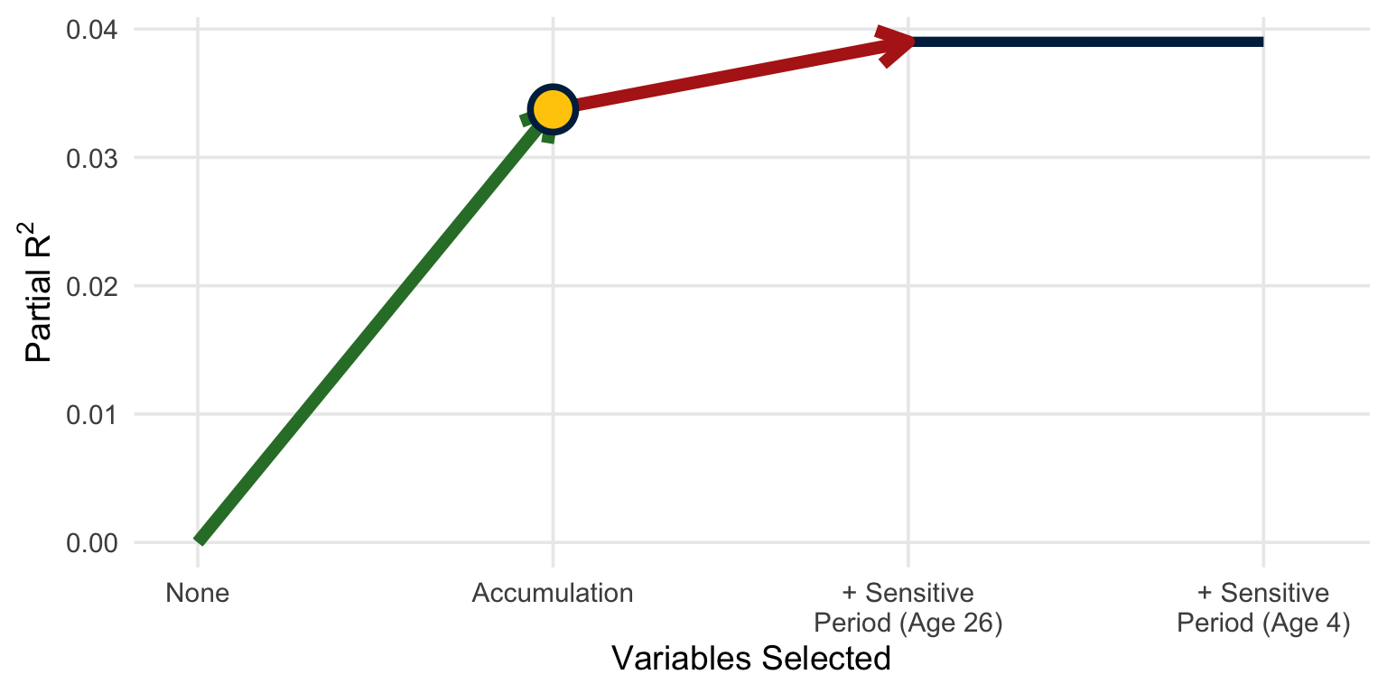
Manual Example Step 2: Compare Model Fit
Are compound hypotheses improving our model?
| Model | Hypothesis | R2 |
|---|---|---|
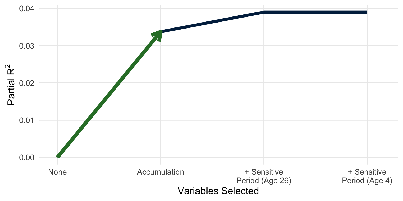
| 1 | Acc | 0.034 |
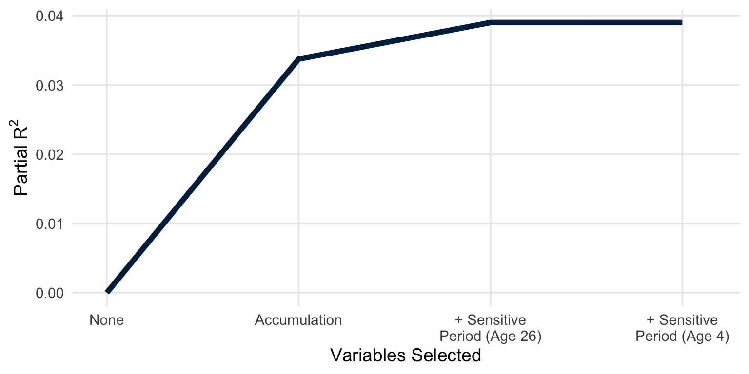
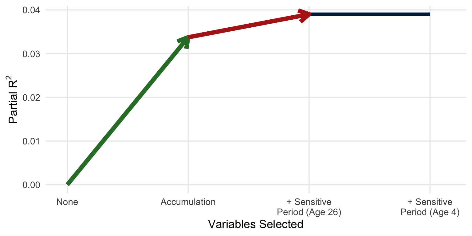
| 2 | Acc + SP26 | 0.039 |
| 3 | Acc + SP26 + SP04 | 0.039 |
Manual Example Step 2: Compare Model Fit
Manual Example Step 2: Compare Model Fit
Manual Example Step 2: Compare Model Fit
Manual Example Step 2: Compare Model Fit
Manual Example Step 3: Calculate Correct p-Value
Call:
lm(formula = y ~ acc, data = dats_bin)

Residuals:
    Min      1Q  Median      3Q     Max
-21.771  -3.318  -0.039   3.160  20.029

Coefficients:
            Estimate Std. Error t value Pr(>|t|)
(Intercept)  29.1837     0.3376  86.433  < 2e-16 ***
acc          -0.9642     0.1566  -6.158 1.04e-09 ***
---
Signif. codes:  0 '***' 0.001 '**' 0.01 '*' 0.05 '.' 0.1 ' ' 1

Residual standard error: 5.215 on 1086 degrees of freedom
Multiple R-squared:  0.03373,   Adjusted R-squared:  0.03285
F-statistic: 37.92 on 1 and 1086 DF,  p-value: 1.039e-09
Manual Example Step 3: Calculate Correct p-Value
- The \(p\)-value in our output \(\left(p = 1.04 \times 10^{-9} \right)\) is incorrect.
- Assumes we only tested a single hypothesis when we actually tested five.
- Easiest way to address this is with a Bonferroni correction.
\[5\left(1.04 \times 10^{-9} \right) = 5.19 \times 10^{-9}\]
Part 4 The slcma Package
A Better Way
- As James Ingram said, “There’s gotta be a better way.”
- The
slcmaR package simplifies everything.
SLCMA Steps with the Package
Manually
With slcma
1. Fit Models
Fit a model for each hypothesis, as well as compound hypotheses
Uses LARS, a more cautious version of forward selection
2. Compare Model Fit
Create an elbow plot
Generates an elbow plot with a single command
3. Calculate p-Values
Apply a Bonferroni correction
Uses fixed LASSO inference or max-|t| test to correct p-values
Installing the Package
- The
slcmapackage is available on GitHub - Can be installed with the
install_github()command from theremotespackage
Install and Load
# install the package
remotes::install_github("thedunnlab/slcma")

# load the package
library(slcma)
Example 1 · Binary Exposures Step 1: Fit Models
Fit All Hypotheses with LARS
slcma_model <- slcma(
  y ~ sp04 + sp26 + sp43 +
    Accumulation(sp04, sp26, sp43) +
    Recency(weights = c(4, 26, 43), sp04, sp26, sp43),
  data = dats_bin
)
Term Role
(Intercept) Adjusted for in all models
sp04 Available for variable selection
sp26 Available for variable selection
sp43 Available for variable selection
Accumulation(sp04, sp26, sp43) Available for variable selection
Recency(weights = c(4, 26, 43), sp04, sp26, sp43) Available for variable selectionExample 1 · Binary Exposures Step 2: Compare Model Fit
Summarize the Selection Path
summary(slcma_model)
Summary of LARS procedure
 Step              Variable selected Variable removed Variables R-squared
    0                                                         0     0.000
    1 Accumulation(sp04, sp26, sp43)                          1     0.022
    2                           sp04                          2     0.029
3 sp43 3 0.039Example 1 · Binary Exposures Step 2: Compare Model Fit
Elbow Plot
plot(slcma_model)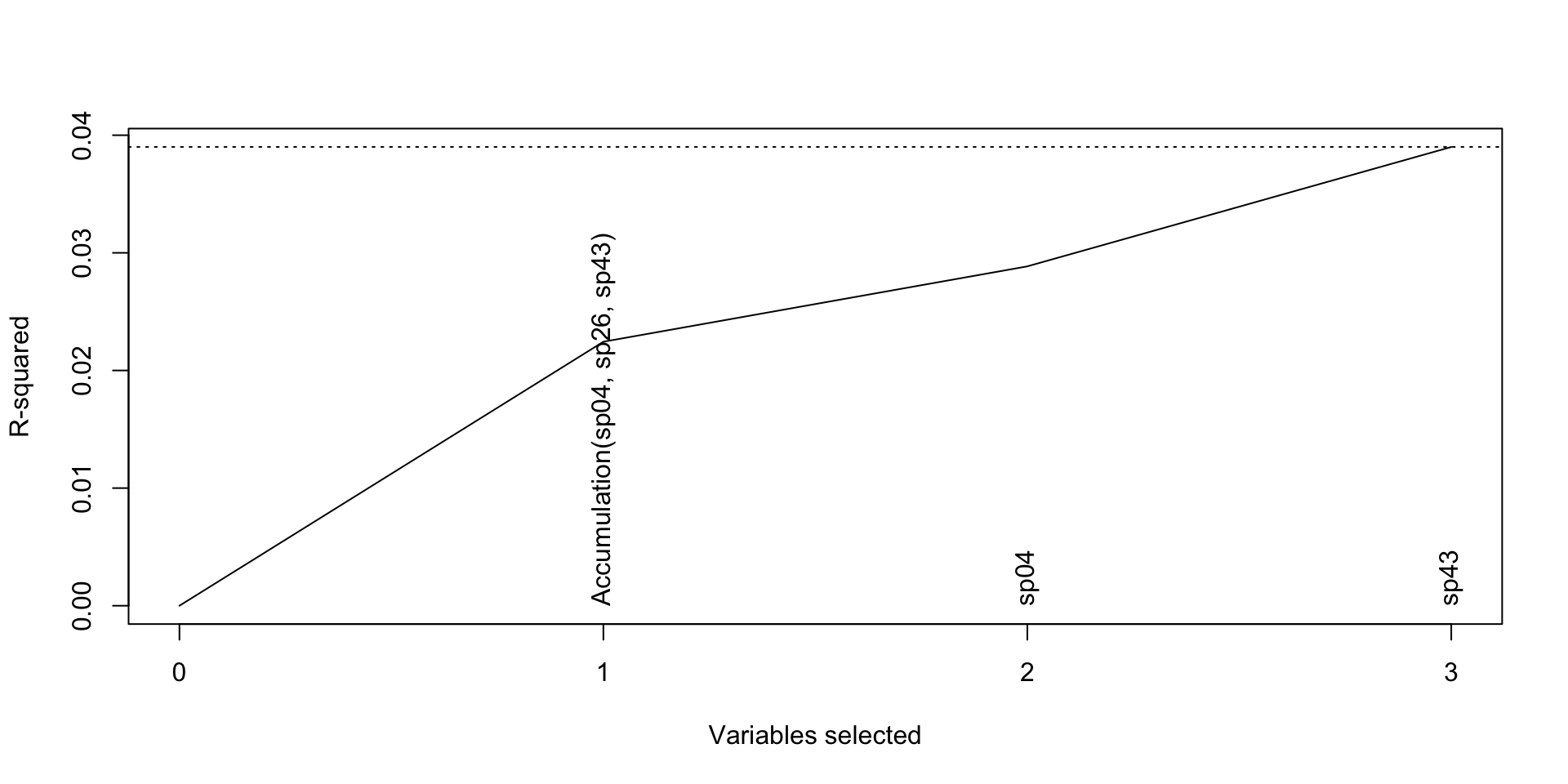
Example 1 · Binary Exposures Step 3: Calculate Correct p-Value
Fixed LASSO Inference
slcmaInfer(slcma_model, 1, method = "slcmaFLI")
Inference for model at Step 1 of LARS procedure

Number of selected variables: 1
R-squared from lasso fit: 0.022

Results from fixed lasso inference (selective inference):

Standard deviation of noise (specified or estimated) sigma = 5.210

Testing results at lambda = 18.578, with alpha = 0.050

                                 Coef P-value  CI.lo CI.up LoTailArea
Accumulation(sp04, sp26, sp43) -0.964       0 -1.272 -0.63      0.024
                               UpTailArea
Accumulation(sp04, sp26, sp43)      0.024
Example 1 · Binary Exposures Parameter Estimates from Relaxed Fit
- What: Ordinary regression refit on the selected hypotheses, with no shrinkage
-
When: Reporting effect sizes (same as the manual
lm(y ~ acc)) - Caution: CIs ignore selection, so take CIs and p-values from Step 3
slcmaInfer(slcma_model, 1, method = "relax")
Inference for model at Step 1 of LARS procedure

Number of selected variables: 1
R-squared from lasso fit: 0.022

Results from relaxed lasso:

R-squared from relaxed lasso fit: 0.034

                                     Coef        SE     CI.lo      CI.up
Accumulation(sp04, sp26, sp43) -0.9641575 0.1562986 -1.270497 -0.6578178
Post-Selection Inference Methods
Naive Calculation
- Inflated FWER
- Biased p-Values
- Fast Computation
Bonferroni Correction
- FWER Controlled
- Unbiased p-Values
- Fast Computation
- Overly Conservative
Fixed LASSO Inference
- FWER Controlled
- Unbiased p-Values
- Slow Computation
Max-|t| Test
- FWER Controlled
- Unbiased p-Values
- Slow Computation
Post-Selection Inference Methods
Fixed LASSO Inference
- Uses
selectiveInferencePackage - 2-Tail CIs; 1-Tail p-Values
- Strange Warnings
Max-|t| Test
- “Baked into”
slcmaPackage - CIs Very Slow
- No Compound Hypotheses
Example 2 · Imputed Data Simulate Example Data
Example 2 · Imputed Data Simulate Example Data
Simulate Complete Data
# set seed
set.seed(1234)

# simulate covariate, hypothesis, and outcome data
n <- 5000
cov1 <- rnorm(n)
cov2 <- rbinom(n, 1, 0.3)
sp1 <- 0.5 * cov1 + rnorm(n)
sp3 <- 0.5 * sp1 + 0.5 * cov1 + rnorm(n)
sp5 <- 0.5 * sp3 + 0.5 * cov1 + rnorm(n)
sp9 <- 0.5 * sp5 + 0.5 * cov1 + rnorm(n)
y <- 0.3 * cov1 + 0.2 * cov2 +
  0.02 * (1 * sp1 + 3 * sp3 + 5 * sp5 + 9 * sp9) + rnorm(n)
Example 2 · Imputed Data Simulate Example Data
Add Missing Values
# set 5% of each covariate and exposure to missing completely at random
cov1[sample(n, 0.05 * n)] <- NA
cov2[sample(n, 0.05 * n)] <- NA
sp1[sample(n, 0.05 * n)] <- NA
sp3[sample(n, 0.05 * n)] <- NA
sp5[sample(n, 0.05 * n)] <- NA
sp9[sample(n, 0.05 * n)] <- NA

# create data frame
dats_miss <- data.frame(cov1, cov2, sp1, sp3, sp5, sp9, y)

# clean up
rm(n, cov1, cov2, sp1, sp3, sp5, sp9, y)
Example 2 · Imputed Data Multiple Imputation
-
Idea: Fill in each missing value several times with plausible draws, creating
mcomplete datasets -
Setup: Impute with the
micepackage, which is installed and loaded withslcma -
In
slcma: Pass the imputed data straight toslcma(), which pools themdatasets into one with their average means and covariances
Example 2 · Imputed Data Impute Data
dats_imp <- mice::mice(
  dats_miss,
  m = 5,
  maxit = 20,
  seed = 4321
)- Include the outcome
yas a predictor in the imputation model - Construct
recandaccafter imputation since they are dependent on imputed values for sensitive periods
Number of Imputations
We use m = 5 for convenience. In practice, use at least as many imputations as the percentage of incomplete cases (26 here; White et al., 2011).
Example 2 · Imputed Data Step 1: Fit Models
Fit All Hypotheses, Adjusting for Covariates
slcma_model <- slcma(
  y ~ cov1 + cov2 + sp1 + sp3 + sp5 + sp9 +
    Accumulation(sp1, sp3, sp5, sp9) +
    Recency(weights = c(1, 3, 5, 9), sp1, sp3, sp5, sp9),
  data = dats_imp,
  adjust = c(1, 2)
)
Term Role
(Intercept) Adjusted for in all models
cov1 Adjusted for in all models
cov2 Adjusted for in all models
sp1 Available for variable selection
sp3 Available for variable selection
sp5 Available for variable selection
sp9 Available for variable selection
Accumulation(sp1, sp3, sp5, sp9) Available for variable selection
Recency(weights = c(1, 3, 5, 9), sp1, sp3, sp5, sp9) Available for variable selectionExample 2 · Imputed Data Step 2: Compare Model Fit
Elbow Plot
plot(slcma_model)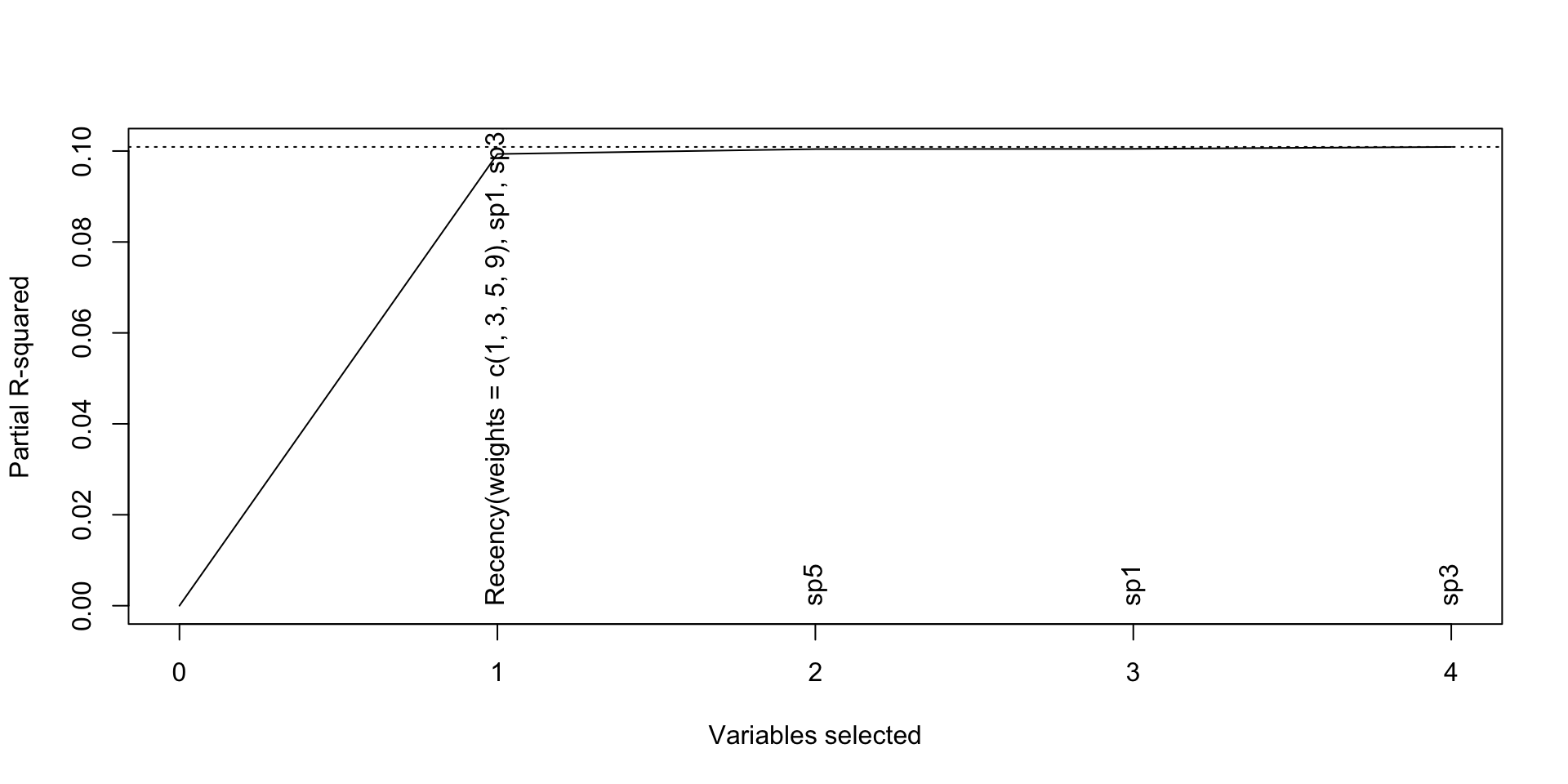
Example 2 · Imputed Data Step 3: Calculate Correct p-Value
Max-|t| Test
slcmaInfer(slcma_model, 1, method = "maxt")
Inference for model at Step 1 of LARS procedure

Number of selected variables: 1
Partial R-squared from lasso fit: 0.099
  Total R-squared from lasso fit: 0.310
Adjusted for: cov1, cov2

Results from max-|t| test:

Error standard deviation: 1.017 on 4993 degrees of freedom

                                                           Coef P-value
Recency(weights = c(1, 3, 5, 9), sp1, sp3, sp5, sp9) 0.02129622       0

Message regarding calculation of P-value: Normal Completion
 with estimated numeric absolute error: 0.000000e+00
Example 2 · Imputed Data Step 3: Calculate Correct p-Value
Max-|t| Test with Confidence Intervals
slcmaInfer(slcma_model, 1, method = "maxt", do.maxtCI = TRUE)
Inference for model at Step 1 of LARS procedure

Number of selected variables: 1
Partial R-squared from lasso fit: 0.099
  Total R-squared from lasso fit: 0.310
Adjusted for: cov1, cov2

Results from max-|t| test:

Error standard deviation: 1.017 on 4993 degrees of freedom
Confidence interval coverage 95.0 percent

                                                           Coef P-value
Recency(weights = c(1, 3, 5, 9), sp1, sp3, sp5, sp9) 0.02129622       0
                                                         CI.lo      CI.up
Recency(weights = c(1, 3, 5, 9), sp1, sp3, sp5, sp9) 0.0207465 0.02349474

Message regarding calculation of P-value: Normal Completion
 with estimated numeric absolute error: 0.000000e+00
Part 5 Important Issues to Keep in Mind
Additional Considerations
Outcome Variables
- Package currently works only for continuous outcomes
Time-Varying Covariates
- SLCMA does not yet accommodate these
- Research is ongoing
- Stick with covariates measured before life course hypotheses
Theory Is Key
SLCMA is not a data mining tool
SLCMA is inseparable from theory
Choose Appropriate Hypotheses
- Each hypothesis tested inflates p-values
- Be parsimonious
Do Not Deviate from Structure
- Some folks like to change their hypotheses after they find null results
- This defeats the purpose of SLCMA
If you want to p-hack, don’t waste your time with SLCMA.
Additional Resources
Foundational Article for SLCMA
Introduction to SLCMA with LARS
Thank You


Please feel free to reach out with questions.
Part 6 · Time Permitting Additional Topics
Additional Topics Additional Hypotheses
Additional Hypotheses Four More Hypotheses
Beyond the Big 3, the slcma package includes helper functions for four more hypotheses.
| Hypothesis | Function | Exposure Type |
|---|---|---|
| Mobility | Mobility(x1, x2) |
Binary only |
| Change | Change(x1, x2) |
Mainly continuous |
| Always Exposed | Always(...) |
Binary only |
| Ever Exposed | Ever(...) |
Binary only |
Additional Hypotheses Mobility \(\left(\mathit{Mob}^{+}_{jk}, \mathit{Mob}^{-}_{jk}\right)\)
- Idea: The direction of change in exposure status between 2 time points, rather than the status at each one, affects the outcome
- Construct: Creates 2 variables: upward (unexposed to exposed) and downward (exposed to unexposed)
- Exposure type: Binary only
\[\mathit{Mob}^{+}_{jk} = \left(1 - x_j\right)x_k \qquad \mathit{Mob}^{-}_{jk} = x_j\left(1 - x_k\right)\]
Additional Hypotheses Mobility \(\left(\mathit{Mob}^{+}_{jk}, \mathit{Mob}^{-}_{jk}\right)\)
Example
| ID | Exp1 | Exp2 | Mob+12 | Mob−12 |
|---|---|---|---|---|
| 1 | 0 | 0 | \((1 - 0) \times 0 = 0\) | \(0 \times (1 - 0) = 0\) |
| 2 | 1 | 1 | \((1 - 1) \times 1 = 0\) | \(1 \times (1 - 1) = 0\) |
| 3 | 0 | 1 | \((1 - 0) \times 1 = 1\) | \(0 \times (1 - 1) = 0\) |
| 4 | 1 | 0 | \((1 - 1) \times 0 = 0\) | \(1 \times (1 - 0) = 1\) |
| 5 | 1 | 0 | \((1 - 1) \times 0 = 0\) | \(1 \times (1 - 0) = 1\) |
Additional Hypotheses Change \(\left(\mathit{Chng}_{jk}\right)\)
- Idea: The change in exposure between 2 time points, rather than the level at each one, affects the outcome
- Construct: Subtract the earlier exposure from the later one
- Exposure type: Mainly continuous
\[\mathit{Chng}_{jk} = x_k - x_j\]
Additional Hypotheses Change \(\left(\mathit{Chng}_{jk}\right)\)
Example
| ID | Exp1 | Exp2 | Chng12 |
|---|---|---|---|
| 1 | 0 | 0 | \(0 - 0 = 0\) |
| 2 | 1 | 1 | \(1 - 1 = 0\) |
| 3 | 0 | 1 | \(1 - 0 = 1\) |
| 4 | 1 | 0 | \(0 - 1 = -1\) |
| 5 | 1 | 0 | \(0 - 1 = -1\) |
Additional Hypotheses Always Exposed \(\left(\mathit{Alw}\right)\)
- Idea: Only exposure that persists across every time point affects the outcome
- Construct: Multiply the exposure variables across time points
- Exposure type: Binary only
\[\mathit{Alw} = \prod_{j=1}^m{x_j}\]
Additional Hypotheses Always Exposed \(\left(\mathit{Alw}\right)\)
Example
| ID | Exp1 | Exp2 | Exp3 | Alw |
|---|---|---|---|---|
| 1 | 0 | 0 | 0 | \(0 \times 0 \times 0 = 0\) |
| 2 | 1 | 1 | 1 | \(1 \times 1 \times 1 = 1\) |
| 3 | 0 | 1 | 0 | \(0 \times 1 \times 0 = 0\) |
| 4 | 1 | 0 | 0 | \(1 \times 0 \times 0 = 0\) |
| 5 | 1 | 0 | 1 | \(1 \times 0 \times 1 = 0\) |
Additional Hypotheses Ever Exposed \(\left(\mathit{Ever}\right)\)
- Idea: Exposure at any time point affects the outcome, regardless of timing or frequency
- Construct: Subtract the product of the non-exposure indicators from 1
- Exposure type: Binary only
\[\mathit{Ever} = 1 - \prod_{j=1}^m{\left(1 - x_j\right)}\]
Additional Hypotheses Ever Exposed \(\left(\mathit{Ever}\right)\)
Example
| ID | Exp1 | Exp2 | Exp3 | Ever |
|---|---|---|---|---|
| 1 | 0 | 0 | 0 | \(1 - (1 \times 1 \times 1) = 0\) |
| 2 | 1 | 1 | 1 | \(1 - (0 \times 0 \times 0) = 1\) |
| 3 | 0 | 1 | 0 | \(1 - (1 \times 0 \times 1) = 1\) |
| 4 | 1 | 0 | 0 | \(1 - (0 \times 1 \times 1) = 1\) |
| 5 | 1 | 0 | 1 | \(1 - (0 \times 1 \times 0) = 1\) |
Additional Hypotheses Any Hypothesis You Can Code
-
How:
slcma()builds its model matrix from the formula, so any term R can compute from your exposures can enter as a hypothesis -
Inline: Wrap arithmetic in
I(), such asI(sp04 * sp26)for exposure at both ages 4 and 26 - Custom Functions: Write a function that takes the exposures and returns one value per person, like the built-in helpers (e.g., peak exposure as the row maximum)
-
Imputed Data: Custom terms are computed within each imputed dataset, just like
Accumulation()andRecency() - Theory First: Each added hypothesis is another candidate in the selection step, so include only those you can justify
Additional Topics Extending SLCMA to New Analyses
Extending SLCMA to New Analyses Beyond Continuous Outcomes
- The
slcmapackage only works with continuous outcomes - What if we want to move beyond this framework?
Use LASSO models with the glmnet package
Use “SLCMA from First Principles”
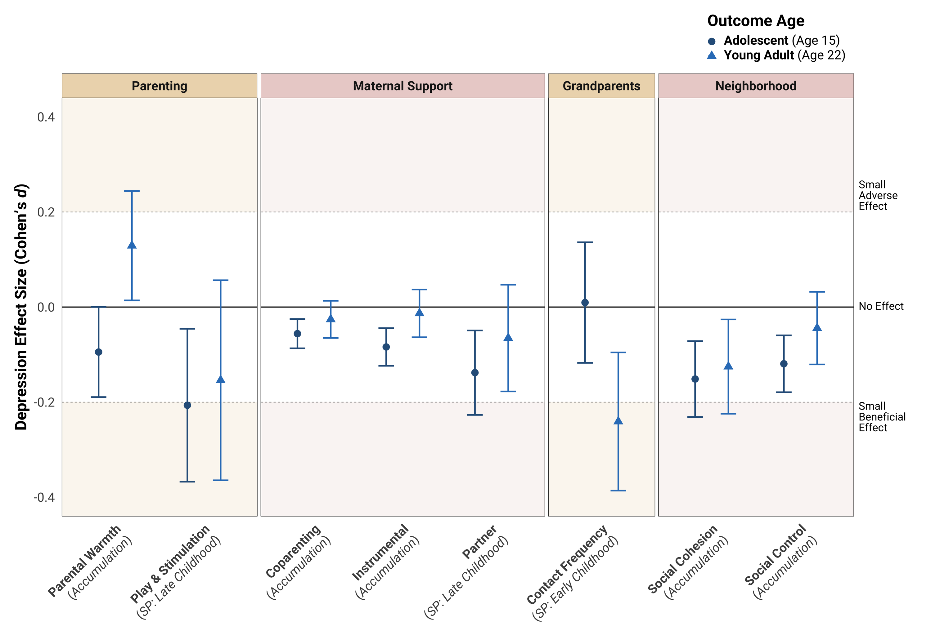
Extending SLCMA to New Analyses Ongoing Research Example
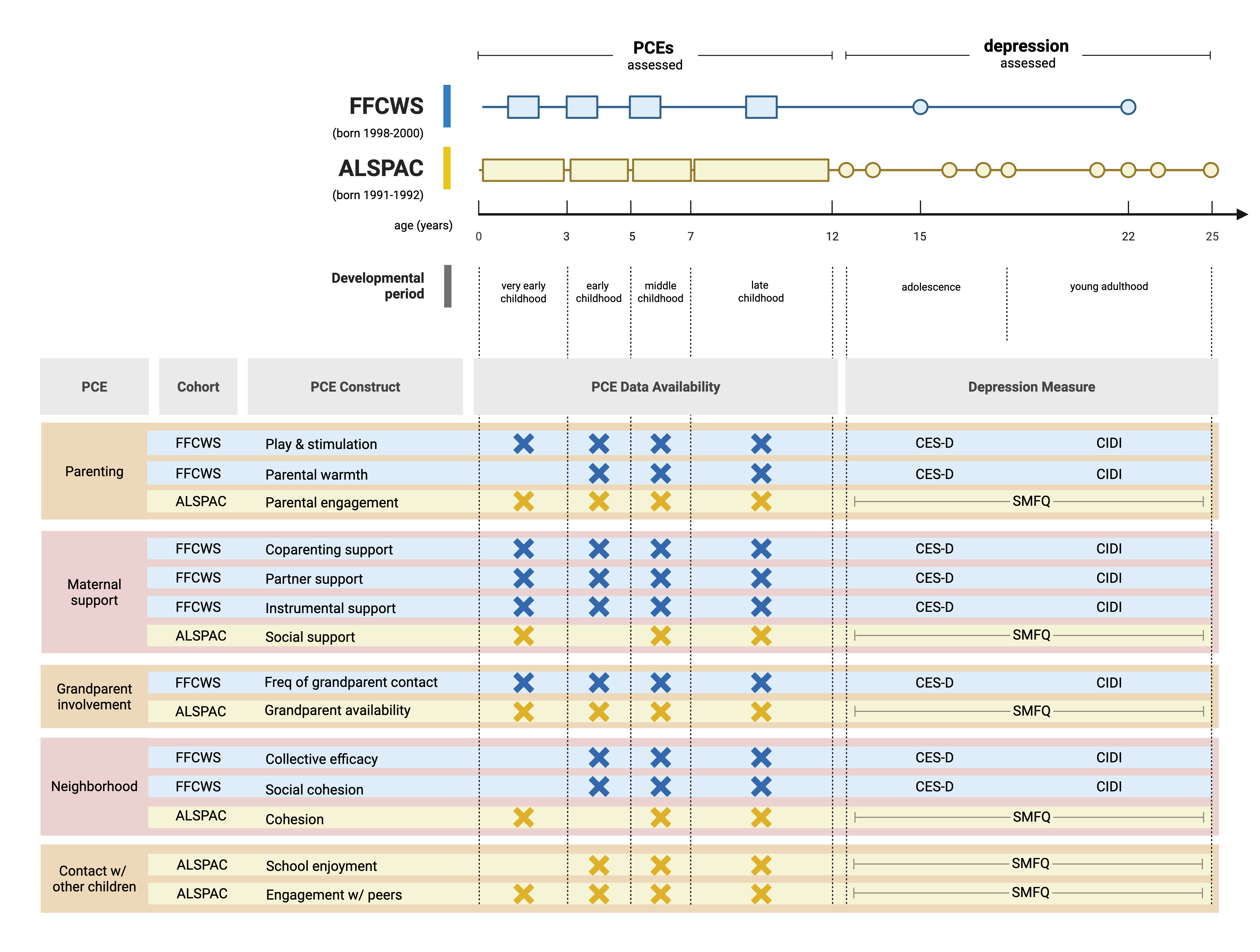
- Title: Positive Childhood Experiences Associate with Lower Depression Risk Throughout Adolescence: Evidence from Two Longitudinal Birth Cohorts
- Research Question: Which life course hypotheses best explain the association between positive childhood experiences (PCEs) and depression trajectories?
ALSPAC
Avon Longitudinal Study of Parents and Children
FFCWS
Future of Families and Child Wellbeing Study
Extending SLCMA to New Analyses Study Design
Extending SLCMA to New Analyses Step 1: Find the Best Hypothesis
Partial Out Covariates
Use the Frisch-Waugh-Lovell theorem:
- \(Y'_{15}\): age 15 depressive symptoms
- \(Y'_{22}\): age 22 depressive criteria
- \(X'_{sp1}\): age 1 sensitive period
- \(X'_{sp3}\): age 3 sensitive period
- \(X'_{sp5}\): age 5 sensitive period
- \(X'_{sp9}\): age 9 sensitive period
- \(X'_{acc}\): accumulation
Compare Hypotheses
Regress each hypothesis on the two depression outcomes:
- \(X'_{sp1} \sim Y'_{15} + Y'_{22}\)
- \(X'_{sp3} \sim Y'_{15} + Y'_{22}\)
- \(X'_{sp5} \sim Y'_{15} + Y'_{22}\)
- \(X'_{sp9} \sim Y'_{15} + Y'_{22}\)
- \(X'_{acc} \sim Y'_{15} + Y'_{22}\)
The model with the largest \(R^2\) is chosen as the best-fitting hypothesis.
Extending SLCMA to New Analyses Step 2: Estimate Coefficients
Regress outcomes on the best-fitting hypothesis to estimate coefficients:
- \(Y_{15} \sim X_{acc} + \text{Covariates}\) (OLS regression)
- \(Y_{22} \sim X_{acc} + \text{Covariates}\) (binary logistic regression)
- \(Y_{22} \sim X_{acc} + Y'_{15} + \text{Covariates}\) (binary logistic regression)
Extending SLCMA to New Analyses Step 3: Global Test p-Values
- Use permutation testing (\(k = 20,000\)) to generate a null distribution for \(R^2\)
- For each permutation, run the full set of regression models and record the highest \(R^2\), irrespective of the hypothesis chosen
- Compare the observed \(R^2\) value to the null distribution to generate a one-tailed \(p\)-value
Extending SLCMA to New Analyses Preliminary Results
Additional Topics Choosing Recency Weights
Choosing Recency Weights Why Weights Are Tricky
- Weights are multiplied by exposures and summed, so they act as quantities of time
- Tricky when waves are unevenly spaced and ages vary within a wave
- Example: Add Health TV hours (Waves I, III, IV, V) predicting happiness at Wave VI
| Age | ||||
|---|---|---|---|---|
| Wave | Years | Range | Mean | Exposure |
| Wave I | 1994-1995 | 12-21 | 15 | tvhrs_1 |
| Wave III | 2001-2002 | 18-26 | 22 | tvhrs_3 |
| Wave IV | 2008-2009 | 24-32 | 28 | tvhrs_4 |
| Wave V | 2016-2018 | 33-43 | 37 | tvhrs_5 |
Choosing Recency Weights Spacing Matters



Choosing Recency Weights Weights Are Quantities, Not Labels
- Recency multiplies and sums the weights, so the arithmetic treats them as amounts
- Analogy: Religious service attendance stored as category codes vs. converted to days per year
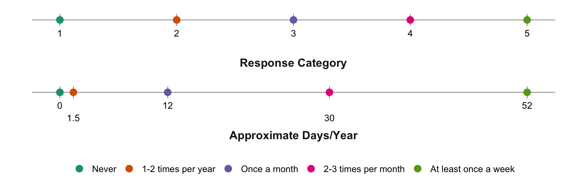
- Wave number is like the category codes, but waves come with a known conversion to time, so use it
Choosing Recency Weights Three Questions to Ask
What is my time metric?
Name it in real units, such as years since baseline or years of age
Does the spacing match the data?
Unequal intervals between waves need unequal intervals between weights
Where does the scale start?
Not at zero, since a weight of 0 drops that occasion from the score
The real test: If you can answer each question in a sentence, you can defend your weights to a reviewer.
Choosing Recency Weights Learn More
- The full tutorial on my website, Choosing Weights for SLCMA Recency Hypothesis, walks through each approach with code and figures.
- Please feel free to reach out with questions.
