Choosing Weights for SLCMA Recency Hypothesis

A guide to choosing recency weights in the SLCMA when panel waves are unequally spaced and respondents vary in age.

One question I’m often asked about the structured life course modeling approach (SLCMA) is how to choose weights for the recency hypothesis. The choice seems straightforward at first, but it gets complicated in panel studies where the waves are unevenly spaced and respondents vary in age within each wave. Below I review the recency hypothesis, work through three options people commonly reach for, and set out what to check before settling on weights for your own data.

If you’re new to the SLCMA, my Presentations page collects several talks I’ve given on the method. For a fuller treatment, see Smith et al. (2022), Statistical Modeling of Sensitive Period Effects Using the Structured Life Course Modeling Approach.

Tips

• All code blocks on this page can be copied by clicking in the upper right corner.
• Note that some code and output blocks may scroll left and right.
• As with all content on my site, please feel free to reach out if you have any questions.

A Review of the Recency Hypothesis

The recency hypothesis assumes that exposures closer in time to the outcome are more strongly associated with it than are more distal exposures. The recency score is calculated as a weighted sum:

\[Rec = \sum^m_{j = 1}\left( x_j \times t_j\right)\]

• \(Rec\): The recency score, one value per participant.
• \(j\): Index for the exposure measurement occasion.
• \(m\): Total number of occasions on which the exposure was measured.
• \(x_j\): Exposure status at occasion \(j\).
• \(t_j\): The recency weight for occasion \(j\).

In the {slcma} package, these values are calculated with the Recency() function. Say we had an exposure measured at ages 4 (sp04), 26 (sp26), and 43 (sp43) years. We can pass those ages to the appropriately named weights argument:

Recency(weights = c(4, 26, 43), sp04, sp26, sp43)

Three Possible Approaches

Say I’m working with the National Longitudinal Study of Adolescent to Adult Health (Add Health) and measuring the exposure at Waves I, III, IV, and V. My exposure variable is the mean hours of TV watched in a typical week, and I want to know how it relates to overall happiness (1-100) at Wave VI, when subjects are 39 to 51 years old.

		Age
Wave	Years	Range	Mean	Exposure
Wave I	1994-1995	12-21	15	tvhrs_1
Wave III	2001-2002	18-26	22	tvhrs_3
Wave IV	2008-2009	24-32	28	tvhrs_4
Wave V	2016-2018	33-43	37	tvhrs_5

A Note on Wave II

You may notice that Wave II is missing here. Dropping it is a common choice with Add Health, since Wave II was fielded only a year after Wave I and excluded the twelfth-grade cohort from Wave I.

Scaling by Wave

The option most people reach for first is to use the wave number as the weight. Here, the weights would be 1, 3, 4, and 5.

In the slcma package, that call looks like this:

Recency(weights = c(1, 3, 4, 5), tvhrs_1, tvhrs_3, tvhrs_4, tvhrs_5)

Once we ask what these weights mean, though, the logic starts to break down. Wave number only works as a metric of time if the waves are evenly spaced, and here they are not.

Scaling by Years Elapsed

A second option is to use the time elapsed between waves. The obvious way to do this is to set the first exposure at 0 and then add the years elapsed at each following wave, giving 0, 7, 13, and 22 years. The trouble is that multiplying the Wave I exposure by zero removes its contribution entirely. Shifting the scale so the first occasion takes a positive value avoids that, so we could use 1, 8, 14, and 23 years instead.

The call would then be:

Recency(weights = c(1, 8, 14, 23), tvhrs_1, tvhrs_3, tvhrs_4, tvhrs_5)

This approach accounts for the unequal intervals between waves, and years elapsed since Wave I is a time metric that is easy to explain in a manuscript.

Scaling by Mean Age in Years

A third option is to use the mean age of subjects at each wave, which is easy enough to implement. The thing to be wary of is that you want these means calculated in your analytic sample. If you’re using listwise deletion, drop the cases with incomplete data before computing them. If you’re using multiple imputation, this matters less. In our example, the values are 15, 22, 28, and 37 years.

The call would be:

Recency(weights = c(15, 22, 28, 37), tvhrs_1, tvhrs_3, tvhrs_4, tvhrs_5)

This works for the same reason the previous approach does. There’s a meaningful time metric underlying the weights, which here is years of age. One caveat is that the mean is only a good stand-in when the age range within a wave is narrow. Here it is not, since Wave I spans nine years, so a weight of 15 misrepresents the oldest respondents by roughly six years. Years elapsed does not have this problem, since every respondent experienced the same interval regardless of their age at baseline.

The Meaning of Time in Recency

You may have noticed that the second and third options held up while the first one did not. The difference is that the second and third rest on an underlying time metric, and wave number does not.

To make this concrete, step outside the recency setting for a moment and consider an analogous situation. Nobody would use religious service attendance as a recency weight, and this is not about how to code an ordinal exposure either. The point is narrower: it is about what happens to any variable when we assign numbers to categories by convention rather than by measurement.

Respondents are asked, “How often do you attend religious services?” and choose from five ordered categories. Those categories are stored in the data file as the integers 1 through 5, but each one can also be translated into an approximate number of days per year.

	Coding
Response	Category	Days/Year
Never	1	0.0
1-2 times per year	2	1.5
Once a month	3	12.0
2-3 times per month	4	30.0
At least once a week	5	52.0

Plotted against each other, the two codings look nothing alike.

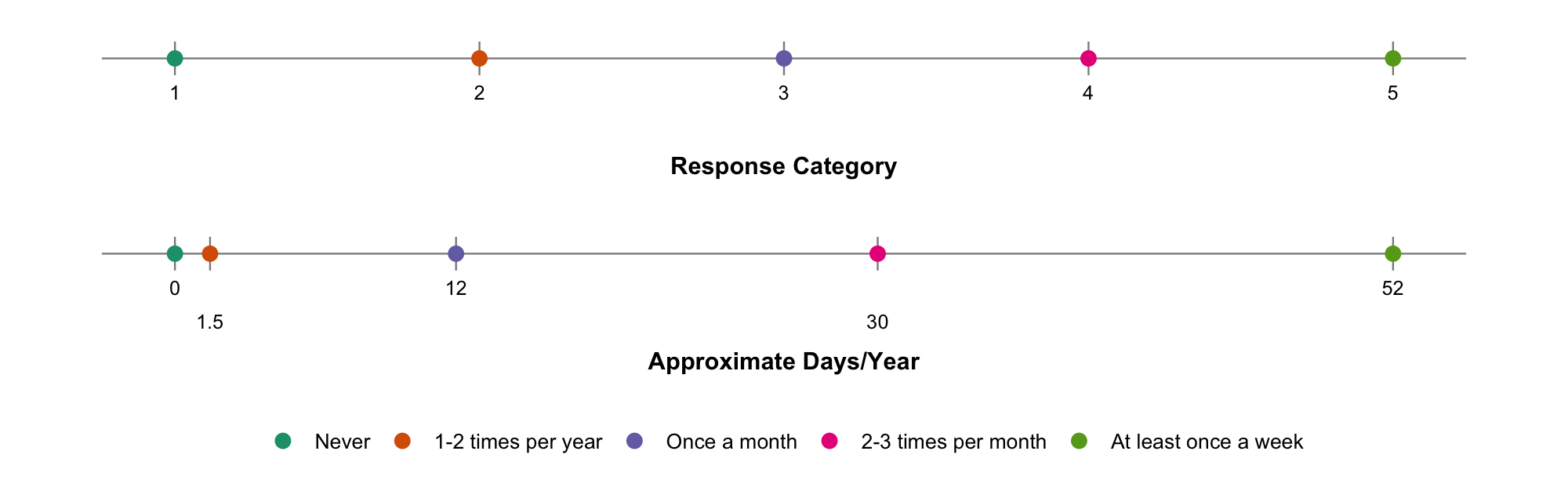
The category codes are evenly spaced because we made them evenly spaced. Nothing about the response options requires the step from “Never” to “1-2 times per year” to match the step from “2-3 times per month” to “At least once a week,” and once we convert to days per year, it clearly does not. Both are single steps in category codes, but one covers about a day and a half while the other covers twenty-two. On the days line the first two categories nearly collide, while the last two sit more than forty percent of the line apart.

Now bring that back to recency. The weights are not merely an ordering. They are multiplied by the exposure and summed, so the arithmetic treats them as quantities. In the attendance example, weighting by the category codes would assert that every step between adjacent categories is the same size, and it would give “Never” a weight of one when the underlying metric says zero.

Wave number is the same kind of variable. It indexes the order of data collection, it is evenly spaced by construction, and it carries no information about how much time passed between waves. The difference is that we are not stuck with it. Unlike the response categories above, waves come with a known conversion, since we know both the years elapsed and the mean age at each one. The recency hypothesis is a claim about time, so the weights should be measured in time.

Final Advice

In my view, choosing recency weights comes down to three questions.

1. What is my time metric? Name it in real units. Years since baseline and years of age both work. If you cannot state your answer as a unit of time, you do not have a metric yet, only an index.
2. Does the spacing match the data? Unequal intervals between waves have to show up as unequal intervals between weights.
3. Where does the scale start? Not at zero. The recency score is a sum of products, so any occasion carrying a weight of zero contributes nothing, and that measurement drops out of the score entirely.

If you can answer all three in a sentence apiece, you can defend the choice to a reviewer, which is usually the real test.